Short Ranged (van der Waals) Potentials

The short ranged pair forces available in DL_POLY_2 are as follows.

1. 12 - 6 potential: (12-6)
   

   $$U(r_{ij})=\left(\frac{A}{r_{ij}^{12}}\right)-\left(\frac{B}{r_{ij}^{6}}\right);$$ (2.70)

   
   

2. Lennard-Jones: (lj)
   

   $$U(r_{ij})=4\epsilon\left[\left (\frac{\sigma}{r_{ij}}\right)^{12}-\left(\frac{\sigma}{r_{ij}}\right)^{6}\right ];$$ (2.71)

   
   

3. n - m potential [27]: (nm)
   

   $$U(r_{ij})=\frac{E_{o}}{(n-m)}\left[m\left (\frac{r_{o}}{r_{ij}}\right)^{n}-n\left(\frac{r_{o}}{r_{ij}}\right)^{m}\right ];$$ (2.72)

   
   

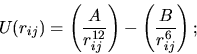
4. Buckingham potential: (buck)
   

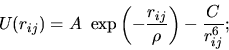   $$U(r_{ij})=A~\exp\left(-\frac{r_{ij}}{\rho}\right)-\frac{C}{r_{ij}^{6}};$$ (2.73)

   
   

5. Born-Huggins-Meyer potential: (bhm)
   

   $$U(r_{ij})=A~\exp[B(\sigma-r_{ij})]-\frac{C}{r_{ij}^{6}}-\frac{D}{r_{ij}^{8}};$$ (2.74)

   
   

6. Hydrogen-bond (12 - 10) potential: (hbnd)
   

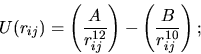   $$U(r_{ij})=\left(\frac{A}{r_{ij}^{12}}\right)-\left(\frac{B}{r_{ij}^{10}}\right);$$ (2.75)

   
   

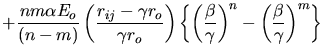
7. Shifted force n - m potential [27]: (snm)
   

   $$U(r_{ij}) = \frac{\alpha E_{o}}{(n-m)}\left [ m\beta^{n}\left \{ \left (\frac... ...r_{o}}{r_{ij}}\right )^{m}- \left(\frac{1}{\gamma}\right)^{m}\right \} \right ]$$

   $$+\frac{nm\alpha E_{o}}{(n-m)} \left ( \frac{r_{ij}-\gamma r_{o}}{... ...frac{\beta}{\gamma}\right )^{n}-\left(\frac{\beta}{\gamma}\right )^{m}\right \}$$ (2.76)

   
   
   with
   

   $$\gamma = \frac{r_{cut}}{r_{o}}$$ (2.77)

   $$\beta = \gamma\left ( \frac{\gamma^{m+1}-1}{\gamma^{n+1}-1} \right ) ^{\frac{1}{n-m}}$$ (2.78)

   $$\alpha = \frac{(n-m)}{[n\beta^{m}(1+(m/\gamma-m-1)/\gamma^{m})- m\beta^{n}(1+(n/\gamma-n-1)/\gamma^{n})]}$$ (2.79)

   
   
   This peculiar form has the advantage over the standard shifted n-m potential in that both $E_{o}$ and $r_{0}$ (well depth and location of minimum) retain their original values after the shifting process.
8. Morse potential: (mors)
   

   $$U(r_{ij})=E_{o}[\{1-\exp(-k(r_{ij}-r_{o}))\}^{2}-1];$$ (2.80)

   
   

9. Tabulation: (tab). The potential is defined numerically only.

The parameters defining these potentials are supplied to DL_POLY_2 at run time (see the description of the FIELD file in section 4.1.3). Each atom type in the system is specified by a unique eight-character label defined by the user. The pair potential is then defined internally by the combination of two atom labels.

As well as the numerical parameters defining the potentials, DL_POLY_2 must also be provided with a cutoff radius $r_{cut}$, which sets a range limit on the computation of the interaction. Together with the parameters, the cutoff is used by the subroutine FORGEN (or FORGEN/SMALL>_RSQ) to construct an interpolation array vvv for the potential function over the range 0 to $r_{cut}$. A second array ggg is also calculated, which is related to the potential via the formula:

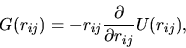$$G(r_{ij})=-r_{ij}\frac{\partial}{\partial r_{ij}}U(r_{ij}),$$ (2.81)

and is used in the calculation of the forces. Both arrays are tabulated in units of energy. The use of interpolation arrays, rather than the explicit formulae, makes the routines for calculating the potential energy and atomic forces very general, and enables the use of user defined pair potential functions. DL_POLY_2 also allows the user to read in the interpolation arrays directly from a file (see the description of the FORTAB routine (chapter 8) and the TABLE file (section 4.1.5). This is particularly useful if the pair potential function has no simple analytical description (e.g. spline potentials).

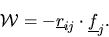
The force on an atom $j$ derived from one of these potentials is formally calculated with the standard formula:

$$\mbox{$\underline{f}$}_{j}=-\frac{1}{r_{ij}}\left[\frac{\par... ...{\partial r_{ij}}U(r_{ij})\right]\mbox{$\underline{r}$}_{ij},$$ (2.82)

where $\mbox{$\underline{r}$}_{ij}=\mbox{$\underline{r}$}_{j}-\mbox{$\underline{r}$}_{i}$. The force on atom $i$ is the negative of this.

The contribution to be added to the atomic virial (for each pair interaction) is

$${\cal W}=-\mbox{$\underline{r}$}_{ij}\cdot\mbox{$\underline{f}$}_{j}.$$ (2.83)

The contribution to be added to the atomic stress tensor is given by

$$\sigma^{\alpha \beta}=r_{ij}^{\alpha}f_{j}^{\beta},$$ (2.84)

where $\alpha$ and $\beta$ indicate the $x,y,z$ components. The atomic stress tensor derived from the pair forces is symmetric.

Since the calculation of pair potentials assumes a spherical cutoff ($r_{cut}$) it is necessary to apply a long range correction to the system potential energy and virial. Explicit formulae are needed for each case and are derived as follows. For two atom types $a$ and $b$, the correction for the potential energy is calculated via the integral

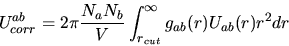$$U_{corr}^{ab}=2\pi \frac{N_{a}N_{b}}{V}\int_{r_{cut}}^{\infty}g_{ab}(r)U_{ab}(r)r^{2}dr$$ (2.85)

where $N_{a},N_{b}$ are the numbers of atoms of types $a$ and $b$, $V$ is the system volume and $g_{ab}(r)$ and $U_{ab}(r)$ are the appropriate pair correlation function and pair potential respectively. It is usual to assume $g_{ab}(r)=1$ for $r>r_{cut}$. DL_POLY_2 sometimes makes the additional assumption that the repulsive part of the short ranged potential is negligible beyond $r_{cut}$.

The correction for the system virial is

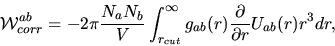$${\cal W}_{corr}^{ab}=-2\pi \frac{N_{a}N_{b}}{V}\int_{r_{cut}}^{\infty}g_{ab}(r)\frac{\partial}{\partial r}U_{ab}(r)r^{3}dr,$$ (2.86)

where the same approximations are applied. Note that these formulae are based on the assumption that the system is reasonably isotropic beyond the cutoff.

In DL_POLY_2 the short ranged forces are calculated by one of the routines SRFRCE, SRFRCE/SMALL>_RSQ, and SRFRCENEU. The long range corrections are calculated by routine LRCORRECT. The calculation makes use of the Verlet neighbour list described above.