![]()
![]()
In the Nosé-Hoover algorithm [18] Newton's
equations of motion are modified to read:
 |
(2.181) |
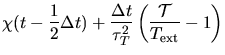
The friction coefficient, ![]() , is controlled by the first order differential equation
, is controlled by the first order differential equation
| (2.182) |
where ![]() is a specified time constant (normally in the range [0.5, 2] ps). In
DL_POLY_2
is a specified time constant (normally in the range [0.5, 2] ps). In
DL_POLY_2
![]() is
stored at half timesteps as it has dimensions of (1/time). The integration takes place as:
is
stored at half timesteps as it has dimensions of (1/time). The integration takes place as:
 |
 |
||
![$\displaystyle {1\over 2} \left[\chi(t-{1\over 2}\Delta t)+\chi(t+{1\over 2}\Delta t)\right]$](img488.png) |
|||
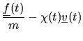
 |
![$\displaystyle \mbox{$\underline{v}$}(t-{1\over 2} \Delta t) +
\Delta t\left[ {\mbox{$\underline{f}$}(t)\over m} -
\chi(t)\mbox{$\underline{v}$}(t)\right]$](img490.png) |
||
![$\displaystyle {1\over 2} \left[\mbox{$\underline{v}$}(t-{1\over 2}\Delta t)
+\mbox{$\underline{v}$}(t+{1\over 2}\Delta t)\right]$](img491.png) |
|||
 |
(2.183) |
Since ![]() is required to calculate
is required to calculate ![]() and itself, the algorithm
requires several iterations to obtain self consistency. In DL_POLY_2 the number of
iterations is set to 3 (4 if the system has bond constraints). The iteration procedure is
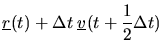
started with the standard Verlet leapfrog prediction of
and itself, the algorithm
requires several iterations to obtain self consistency. In DL_POLY_2 the number of
iterations is set to 3 (4 if the system has bond constraints). The iteration procedure is
started with the standard Verlet leapfrog prediction of ![]() and
and ![]() . The conserved quantity is derived from the
extended Hamiltonian for the system which, to within a constant, is the Helmholtz free
energy:
. The conserved quantity is derived from the
extended Hamiltonian for the system which, to within a constant, is the Helmholtz free
energy:
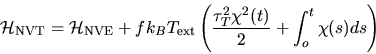 |
(2.184) |
If bond constraints are present an extra iteration is required due to the call to the SHAKE routine. Note that the SHAKE corrections need only be applied during the first iteration as subsequent to this the velocities, relative to the bond c.o.m. velocity, will be orthogonal to the bond vectors. The velocity scaling imposed by the thermostat is isotropic so does not destroy this orthogonality. The algorithm is implemented in the DL_POLY routines NVT_H0 and NVT_H1, the latter being for systems with bond constraints.
![]()