The Hoover Barostat

DL_POLY_2 uses the Melchionna modification of the Hoover algorithm [38] in which the equations of motion involve a Nosé - Hoover thermostat and a barostat in the same spirit.

Cell size variation

For isotropic fluctuations the equations of motion are:

$${d \mbox{$\underline{r}$}(t) \over d t} = \mbox{$\underline{v}$}(t) + \eta(\mbox{$\underline{r}$}(t) - \mbox{$\underline{R}$}_0)$$

$${d \mbox{$\underline{v}$}(t) \over d t} = {\mbox{$\underline{f}$}(t)\over m} - \left[\chi(t)+\eta(t)\right]\mbox{$\underline{v}$}(t)$$

$${d\chi(t) \over dt} = {1 \over \tau_T^2}\left( {{\cal T}\over T_{\rm ext}} - 1\right)$$

$${d\eta(t) \over dt} = {1 \over {\cal N}k_B T_{\rm ext}\tau_P^2} V(t) ({\cal P} - P_{\rm ext})$$

$${d V(t) \over dt} = [3 \eta(t)] V(t)$$ (2.190)

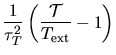
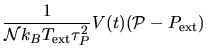
where $\eta$ is the barostat friction coefficient, $R_0$ the system centre of mass, $\tau_P$ a specified time constant for pressure fluctuations, ${\cal P}$ the instantaneous pressure and $V$ the system volume.

The conserved quantity is, to within a constant, the Gibbs free energy of the system:

$${\cal H}_{NPT} = {\cal H}_{NVT} + P_{\rm ext} V(t) + {3 {\cal N} k_B T_{\rm ext} \over 2} \eta(t)^2 \tau_P^2$$ (2.191)

The algorithm is readily implemented in the leapfrog scheme:

$$\chi(t+{1\over2}\Delta t) \leftarrow \chi(t-{1\over 2}\Delta t) + {\Delta t \over \tau_T^2}\left( {{\cal T}\over T_{\rm ext}} - 1\right)$$

$$\chi(t) \leftarrow {1\over 2} \left[\chi(t-{1\over 2}\Delta t)+\chi(t+{1\over 2}\Delta t)\right]$$

$$\eta(t+{1\over2}\Delta t) \leftarrow \eta(t-{1\over 2}\Delta t) + {\Delta t V(t) \over {\cal N} k_B T_{\rm ext} \tau_P^2}\left( {{\cal P} - P_{\rm ext}}\right)$$

$$\eta(t) \leftarrow {1\over 2} \left[\eta(t-{1\over 2}\Delta t)+\eta(t+{1\over 2}\Delta t)\right]$$

$$\mbox{$\underline{v}$}(t + {1\over 2} \Delta t) \leftarrow \mbox{$\underline{v}$}(t-{1\over 2} \Delta t) + \Delta t\left[ {\... ...{f}$}(t)\over m} - \left[\chi(t)+\eta(t)\right]\mbox{$\underline{v}$}(t)\right]$$

$$\mbox{$\underline{v}$}(t) \leftarrow {1\over 2} \left[\mbox{$\underline{v}$}(t-{1\over 2}\Delta t) +\mbox{$\underline{v}$}(t+{1\over 2}\Delta t)\right]$$

$$\mbox{$\underline{r}$}(t+\Delta t) \leftarrow \mbox{$\underline{r}$}(t) + \Delta t \left(\mbox{$\underline{v}$}... ...x{$\underline{r}$}(t+{1\over 2}\Delta t)-\mbox{$\underline{R}$}_0\right]\right)$$

$$\mbox{$\underline{r}$}(t+{1\over 2}\Delta t) \leftarrow {1\over 2} \left[ \mbox{$\underline{r}$}(t)+ \mbox{$\underline{r}$}(t+\Delta t)\right]$$ (2.192)

Like the Nosé-Hoover thermostat, several iterations are required to obtain self consistency. DL_POLY_2 uses 4 iterations (5 if bond constraints are present) with the standard Verlet leapfrog predictions for the initial estimates of ${\cal T}$, ${\cal P}$, $\mbox{$\underline{v}$}(t)$ and $\mbox{$\underline{r}$}(t+{1\over 2}\Delta t)$. Note also that the change in box size requires the SHAKE algorithm to be called each iteration with the new cell vectors obtained from:

$$V(t+\Delta t) \leftarrow V(t) \exp\left[3\Delta t\; \eta(t+{1\over 2}\Delta t)\right]$$

$$\mbox{$\underline{\underline{\bf H}}$}(t+\Delta t) \leftarrow \mbox{$\underline{\underline{\bf H}}$}(t)\exp\left[\Delta t \;\eta(t+{1\over 2}\Delta t)\right]$$ (2.193)

where $\underline{\underline{\bf H}}$ is the cell matrix whose columns are the three cell vectors $\mbox{$\underline{a}$},\mbox{$\underline{b}$},\mbox{$\underline{c}$}$.

The isotropic changes to cell volume are implemented in the DL_POLY routine NPT_H1 which allows for systems containing bond constraints.

Cell size and shape variation

The isotropic algorithm may be extended to allowing the cell shape to vary by defining $\eta$ as a tensor, $\underline{\underline{\bf\eta}}$. The equations of motion are implemented as:

$$\chi(t+{1\over2}\Delta t) \leftarrow \chi(t-{1\over 2}\Delta t) + {\Delta t \over \tau_T^2}\left( {{\cal T}\over T_{\rm ext}} - 1\right)$$

$$\chi(t) \leftarrow {1\over 2} \left[\chi(t-{1\over 2}\Delta t)+\chi(t+{1\over 2}\Delta t)\right]$$

$$\mbox{$\underline{\underline{\bf\eta}}$}(t+{1\over2}\Delta t) \leftarrow \mbox{$\underline{\underline{\bf\eta}}$}(t-{1\over 2}\Delta t) + ... ...erline{\bf\sigma}}$} - P_{\rm ext}\mbox{$\underline{\underline{\bf 1}}$}\right)$$

$$\mbox{$\underline{\underline{\bf\eta}}$}(t) \leftarrow {1\over 2} \left[\mbox{$\underline{\underline{\bf\eta}}$}(t-{1\ov... ...Delta t)+ \mbox{$\underline{\underline{\bf\eta}}$}(t+{1\over 2}\Delta t)\right]$$

$$\mbox{$\underline{v}$}(t + {1\over 2} \Delta t) \leftarrow \mbox{$\underline{v}$}(t-{1\over 2} \Delta t) + \Delta t\left[ {\... ...ox{$\underline{\underline{\bf\eta}}$}(t)\right]\mbox{$\underline{v}$}(t)\right]$$

$$\mbox{$\underline{v}$}(t) \leftarrow {1\over 2} \left[\mbox{$\underline{v}$}(t-{1\over 2}\Delta t) +\mbox{$\underline{v}$}(t+{1\over 2}\Delta t)\right]$$

$$\mbox{$\underline{r}$}(t+\Delta t) \leftarrow \mbox{$\underline{r}$}(t) + \Delta t \left(\mbox{$\underline{v}$}... ...x{$\underline{r}$}(t+{1\over 2}\Delta t)-\mbox{$\underline{R}$}_0\right]\right)$$

$$\mbox{$\underline{r}$}(t+{1\over 2}\Delta t) \leftarrow {1\over 2} \left[ \mbox{$\underline{r}$}(t)+ \mbox{$\underline{r}$}(t+\Delta t)\right]$$ (2.194)

where $\underline{\underline{\bf 1}}$ is the identity matrix and $\underline{\underline{\bf\sigma}}$ the pressure tensor. The new cell vectors are calculated from

$$\mbox{$\underline{\underline{\bf H}}$}(t+\Delta t) \leftarrow \mbox{$\underline{\underline{\bf H}}$}(t)\exp\left[\Delta t \;\mbox{$\underline{\underline{\bf\eta}}$}(t+{1\over 2}\Delta t)\right]$$ (2.195)

DL_POLY_2 uses a power series expansion truncated at the quadratic term to approximate the exponential of the tensorial term. The new volume is found from

$$V(t+\Delta t) \leftarrow V(t) \exp\left[ \Delta t\; {\rm tr}(\mbox{$\underline{\underline{\bf\eta}}$})\right]$$ (2.196)

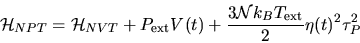
The conserved quantity is

$${\cal H}_{NPT} = {\cal H}_{NVT} + P_{\rm ext} V(t) + {3 {\ca... ...m tr} [\mbox{$\underline{\underline{\bf\eta}}$}(t)]^2 \tau_P^2$$ (2.197)

This algorithm is implemented in the routines NST_H0 (nonbonded systems) and NST_H1 (with bond constraints).