


Next: Rigid Bodies and Rotational
Up: Barostats
Previous: The Hoover Barostat
Contents
Index
With the Berendsen barostat the system is made to obey the equation of motion
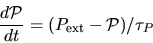 |
(2.198) |
Cell size variations
In the isotropic implementation, at each step the MD cell volume is
scaled by by a factor  and the coordinates, and cell vectors, by
 where
where
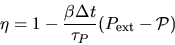 |
(2.199) |
and  is the isothermal compressibility of the system.
The Berendesen thermostat is applied at the same time.
In practice is a specified constant
which DL_POLY_2 takes to be the isothermal compressibility of liquid water.
The exact value is not critical to the algorithm
as it relies on the ratio
is the isothermal compressibility of the system.
The Berendesen thermostat is applied at the same time.
In practice is a specified constant
which DL_POLY_2 takes to be the isothermal compressibility of liquid water.
The exact value is not critical to the algorithm
as it relies on the ratio  .
.  is specified by the user.
This algorithm is implemented in NPT_B1 with 4 or 5 iterations
used to obtain self consistency in the
 .
.
Cell size and shape variations
The extension of the isotropic algorithm to anisotropic cell
variations is straightforward. The tensor
 is defined by
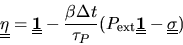 |
(2.200) |
and the new cell vectors given by
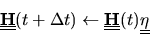 |
(2.201) |
As in the isotropic case the Berendsen thermostat is applied simultaneously and 4 or 5 iterations are
used to obtain convergence.
The algorithm is implemented in NST_B0 (nonbonded systems) and
NST_B1 (with bond constraints).
Next: Rigid Bodies and Rotational
Up: Barostats
Previous: The Hoover Barostat
Contents
Index
W Smith
2003-05-12