![]()
![]()
The Ewald sum [12] is the best technique for calculating electrostatic interactions in a periodic (or pseudo-periodic) system.
The basic model for a neutral periodic system is a system of charged point ions mutually interacting via the Coulomb potential. The Ewald method makes two amendments to this simple model. Firstly each ion is effectively neutralised (at long range) by the superposition of a spherical gaussian cloud of opposite charge centred on the ion. The combined assembly of point ions and gaussian charges becomes the Real Space part of the Ewald sum, which is now short ranged and treatable by the methods described above (section 2.1). 2.3 The second modification is to superimpose a second set of gaussian charges, this time with the same charges as the original point ions and again centred on the point ions (so nullifying the effect of the first set of gaussians). The potential due to these gaussians is obtained from Poisson's equation and is solved as a Fourier series in Reciprocal Space. The complete Ewald sum requires an additional correction, known as the self energy correction, which arises from a gaussian acting on its own site, and is constant. Ewald's method therefore replaces a potentially infinite sum in real space by two finite sums: one in real space and one in reciprocal space; and the self energy correction.
For molecular systems, as opposed to systems comprised simply of point ions, additional
modifications are necessary to correct for the excluded (intra-molecular) Coulombic
interactions. In the real space sum these are simply omitted. In reciprocal space however,
the effects of individual gaussian charges cannot easily be extracted,
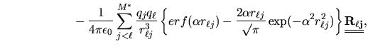
and the correction is made in real space. It amounts to removing terms corresponding to
the potential energy of an ion ![]() due to the gaussian charge on a
neighbouring charge
due to the gaussian charge on a
neighbouring charge ![]() (or vice versa). This correction appears as the final term in the full
Ewald formula below. The distinction between the error function
(or vice versa). This correction appears as the final term in the full
Ewald formula below. The distinction between the error function ![]() and the
more usual complementary error function
and the
more usual complementary error function ![]() found in the real space sum, should be noted.
found in the real space sum, should be noted.
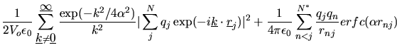
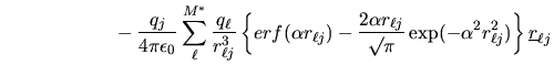
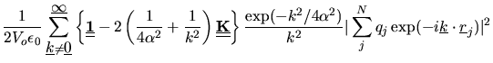
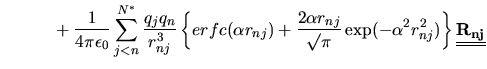
The total electrostatic energy is given by the following formula.
 |
|||
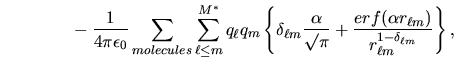 |
(2.131) |
where ![]() is the number of ions in the system and
is the number of ions in the system and ![]() the same number discounting any excluded
(intramolecular) interactions.
the same number discounting any excluded
(intramolecular) interactions. ![]() represents the number of excluded atoms in a given
molecule and includes the atomic self correction.
represents the number of excluded atoms in a given
molecule and includes the atomic self correction. ![]() is the simulation cell volume
and
is the simulation cell volume
and ![]() is a reciprocal lattice vector defined by
is a reciprocal lattice vector defined by
where ![]() are integers and
are integers and ![]() are the reciprocal
space basis vectors. Both
are the reciprocal
space basis vectors. Both ![]() and
and ![]() are derived
from the vectors (
are derived
from the vectors ( ![]() ) defining
the simulation cell. Thus
) defining
the simulation cell. Thus
| (2.133) |
and
 |
|||
 |
(2.134) | ||
 |
With these definitions, the Ewald formula above is applicable to general periodic systems. (A small additional modification is necessary for rhombic dodecahedral and truncated octahedral simulation cells [30].)
In practice the convergence of the Ewald sum is controlled by three variables: the real
space cutoff ![]() ; the convergence parameter
; the convergence parameter ![]() and the largest reciprocal space vector
and the largest reciprocal space vector ![]() used in the reciprocal space sum. These are
discussed more fully in section 3.3.5. DL_POLY_2 can
provide estimates if requested (see CONTROL file description 4.1.1.
used in the reciprocal space sum. These are
discussed more fully in section 3.3.5. DL_POLY_2 can
provide estimates if requested (see CONTROL file description 4.1.1.
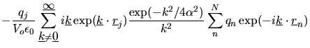
The force on an atom ![]() is obtained by differentiation and is
is obtained by differentiation and is
 |
|||
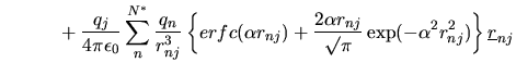 |
(2.135) | ||
 |
The electrostatic contribution to the system virial can be obtained as the negative of the Coulombic energy. However in DL_POLY_2 this formal equality can be used as a check on the convergence of the Ewald sum. The actual electrostatic virial is obtained during the calculation of the diagonal of the stress tensor.
The electrostatic contribution to the stress tensor is given by
 |
|||
 |
(2.136) | ||
 |
where matrices ![]() and
and ![]() are defined as follows.
are defined as follows.
| (2.137) | |||
| (2.138) |
In DL_POLY_2 the full Ewald sum is handled by several routines: EWALD1 and EWALD1A handle the reciprocal space terms; EWALD2, EWALD2_3PT, EWALD2_RSQ and EWALD4, EWALD4_3PT handle the real space terms (with the same Verlet neighbour list routines that are used to calculate the short range forces); and EWALD3 calculates the self interaction corrections. It should be noted that the Ewald potential and force interpolation arrays in DL_POLY_2 are erc and fer respectively.
![]()