![]()
![]()
As its name implies the Smoothed Particle Mesh Ewald (SPME) method
is a modification of the standard Ewald method. DL_POLY_2 implements the SPME method of
Essmann et al. [31]. Formally this method
is capable of treating van der Waals forces also, but in DL_POLY_2 it is confined to
electrostatic forces only. The main difference from the standard Ewald method is in its
treatment of the the reciprocal space terms. By means of an interpolation procedure
involving (complex) B-splines, the sum in reciprocal space is represented on a three
dimensional rectangular grid. In this form the Fast Fourier Transform (FFT) may be used to
perform the primary mathematical operation, which is a 3D convolution. The efficiency of
these procedures greatly reduces the cost of the reciprocal space sum when the range of ![]() vectors is large. The method (briefly) is as follows (for
full details see [31]):
vectors is large. The method (briefly) is as follows (for
full details see [31]):
 |
(2.139) |
in which ![]() is the integer index of the
is the integer index of the ![]() vector in a principal
direction,
vector in a principal
direction, ![]() is the total number of grid points in the same direction and
is the total number of grid points in the same direction and ![]() is the fractional
coordinate of ion
is the fractional
coordinate of ion ![]() scaled by a factor
scaled by a factor ![]() (i.e.
(i.e. ![]() ). Note that the definition of the B-splines
implies a dependence on the integer
). Note that the definition of the B-splines
implies a dependence on the integer ![]() , which limits the formally infinite sum over
, which limits the formally infinite sum over ![]() . The coefficients
. The coefficients ![]() are
B-splines of order
are
B-splines of order ![]() and the factor
and the factor ![]() is a constant computable from the formula:
is a constant computable from the formula:
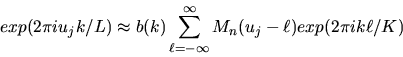
![\begin{displaymath}
b(k)=exp(2\pi i (n-1)k/K)\left
[\sum_{\ell=0}^{n-2} M_{n}(\ell+1) exp(2\pi i k\ell/K)\right ]^{-1}
\end{displaymath}](img337.png) |
(2.140) |
| (2.141) |
where ![]() is the discrete Fourier transform of the charge
array
is the discrete Fourier transform of the charge
array ![]() defined as
defined as
 |
(2.142) |
(in which the sums over ![]() etc are required to capture contributions from all
relevant periodic cell images, which in practice means the nearest images.)
etc are required to capture contributions from all
relevant periodic cell images, which in practice means the nearest images.)
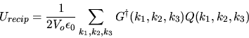 |
(2.143) |
in which ![]() is the discrete Fourier transform of the function
is the discrete Fourier transform of the function
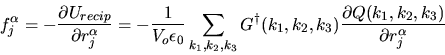
| (2.144) |
and where
| (2.145) |
and ![]() is the complex conjgate of
is the complex conjgate of ![]() . The function
. The function ![]() is thus a
relatively simple product of the gaussian screening term appearing in the conventional
Ewald sum, the function
is thus a
relatively simple product of the gaussian screening term appearing in the conventional
Ewald sum, the function ![]() and the discrete Fourier transform of
and the discrete Fourier transform of ![]()
 |
(2.146) |
Fortunately, due to the recursive properties of the B-splines, these formulae are easily evaluated.
The virial and the stress tensor are calculated in the same manner as for the conventional Ewald sum.
The DL_POLY_2 subroutines required to calculate the SPME contributions are:
BSPGEN, which calculates the B-splines; BSPCOE, which
calculates B-spline coefficients; SPL_CEXP, which calculates the FFT and
B-spline complex exponentials; EWALD_SPME, which calculates the reciprocal
space contributions; SPME_FOR, which calculates the reciprocal space
forces; and DLPFFT3, which calculates the 3D complex fast Fourier transform
(default code only, Cray, SGI, IBM SP machines have their own FFT routines, selected at
compile time and the FFTW public FFT is also an option). These subroutines calculate the
reciprocal space components of the Ewald sum only, the real-space calculations are
performed by EWALD2, EWALD3 and EWALD 4, as
for the normal Ewald sum. In addition there are a few minor utility routines : CPY_RTC
copies a real array to a complex array; ELE_PRD is an element-for-element
product of two arrays; SCL_CSUM is a scalar sum of elements of a complex
array; and SET_BLOCK initialises an array to a present value (usually
zero).
![]()