Next: Reaction Field
Up: Long Ranged Electrostatic (Coulombic)
Previous: Smoothed Particle Mesh Ewald
Contents
Index
Hautman Klein Ewald (HKE)
The method of Hautman and Klein is an adaptation of the Ewald method
for systems which are periodic in two dimensions only
[32]. (DL_POLY_2 assumes this periodicity is in the XY plane.)
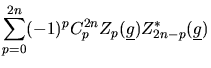
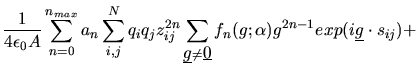
The HKE method gives the following formula for the electrostatic
energy of a system of  (nonbonded) ions that is overall charge
neutral2.4:
(nonbonded) ions that is overall charge
neutral2.4:
In this formula  is the system area (in the
XY plane),
is the system area (in the
XY plane),
 is a 2D lattice vector representing the 2D
periodicity of the system,
is a 2D lattice vector representing the 2D
periodicity of the system,  is the in-plane (XY) component of
the interparticle distance
is the in-plane (XY) component of
the interparticle distance  and
and
 is a reciprocal
lattice vector. Thus
is a reciprocal
lattice vector. Thus
 |
(2.148) |
where
 are integers and vectors
 and
and
 are the lattice basis vectors. The reciprocal lattice vectors are:
 |
(2.149) |
where  are integers
 are reciprocal space
vectors (defined in terms of the vectors
and
):
are reciprocal space
vectors (defined in terms of the vectors
and
):
The functions
 and
and
 are the HKE
convergence functions, in real and reciprocal space respectively.
(C.f. the complementary error and gaussian functions of the original
Ewald method.) However they occur to higher orders here, as indicated
by the sum over subscript
are the HKE
convergence functions, in real and reciprocal space respectively.
(C.f. the complementary error and gaussian functions of the original
Ewald method.) However they occur to higher orders here, as indicated
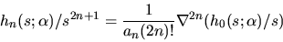
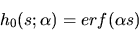
by the sum over subscript  , which corresponds to terms in a Taylor
expansion of
, which corresponds to terms in a Taylor
expansion of  in
in  , the in-plane distance
[32]. Usually this sum is truncated at
, the in-plane distance
[32]. Usually this sum is truncated at  , but
in DL_POLY_2 can go as high as
, but
in DL_POLY_2 can go as high as  . In the HKE method the
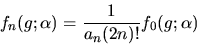
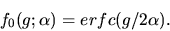
convergence functions are defined as follows:
. In the HKE method the
convergence functions are defined as follows:
 |
(2.151) |
with
 |
(2.152) |
and
 |
(2.153) |
with
 |
(2.154) |
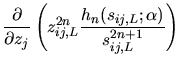
In DL_POLY_2 the
 functions are derived by a
recursion algorithm, while the
functions are derived by a
recursion algorithm, while the
 functions are
obtained by direct evaluation. The coefficients
functions are
obtained by direct evaluation. The coefficients  are given by
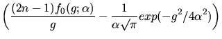
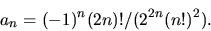 |
(2.155) |
As pointed out by Hautman and Klein, the equation (2.147) allows
separation of the  components via the binomial expansion,
which greatly simplifies the double sum over atoms
in reciprocal space. Thus the reciprocal space part of equation
(2.147) becomes
components via the binomial expansion,
which greatly simplifies the double sum over atoms
in reciprocal space. Thus the reciprocal space part of equation
(2.147) becomes
 |
(2.156) |
with  a binomial coefficient and
 |
(2.157) |
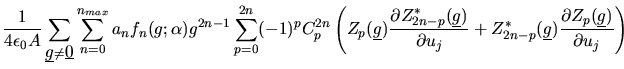
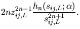
The force on an ion is obtained by the usual differentiation, however
in this case the z components have different expressions from the x
and y.
where  is one of
 and (noting for brevity
that
and (noting for brevity
that  and
and  derivatives are similar)
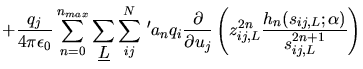
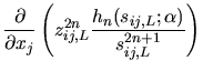
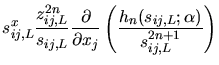
and
In DL_POLY_2 the partial derivatives of
 are calculated by a recursion algorithm. Note that when
  there is
no derivative w.r.t.
there is
no derivative w.r.t.  .
.
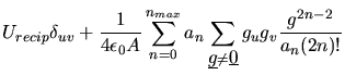
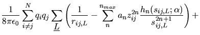
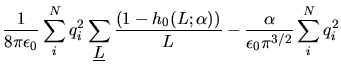
The virial and stress tensor terms in real space may be calculated
directly from the pair forces and interatomic distances in the usual
way, and need not be discussed further. The calculation of the
reciprocal space contributions (the terms involving the
functions) are more difficult. Firstly however we
note that the reciprocal space contributions to
 and
and
 may be obtained directly from the force calculations
thus:
may be obtained directly from the force calculations
thus:
which renders the calculation of these components trivial. The
remaining components are calculated from
where  are one or both of the components
  . Note that,
although it is possible to define these contributions to the stress
tensor, it is not possible to calculate a pressure from them unless a
finite, arbitrary boundary is imposed on the z direction (which is an
assumption applied in DL_POLY_2 , but without implications of periodicity in
the z-direction). The components define the surface tension
however.
. Note that,
although it is possible to define these contributions to the stress
tensor, it is not possible to calculate a pressure from them unless a
finite, arbitrary boundary is imposed on the z direction (which is an
assumption applied in DL_POLY_2 , but without implications of periodicity in
the z-direction). The components define the surface tension
however.
For bonded molecules, as with the standard 3D Ewald sum, it is
necessary to extract contributions associated with the excluded atom
pairs. In the DL_POLY_2 HKE implementation this amounts to an a
posteriori subtraction of the corresponding coulomb terms.
In DL_POLY_2 the HKE method is handled by several subroutines: HKGEN
constructs the
convergence functions and their
derivatives; HKEWALD1 calculates the reciprocal space terms;
HKEWALD2 and HKEWALD3 calculate the real space terms and
the bonded atom corrections respectively. HKEWALD4 calculates
the primary interactions in the multiple timestep implementation.
Next: Reaction Field
Up: Long Ranged Electrostatic (Coulombic)
Previous: Smoothed Particle Mesh Ewald
Contents
Index
W Smith
2003-05-12