


Next: Linked Rigid Bodies
Up: Rigid Bodies and Rotational
Previous: Description of Rigid Body
Contents
Index
The net translational force acting upon the rigid unit is
 |
(2.204) |
where
 is the force on a rigid unit site, and the sum includes
all sites
is the force on a rigid unit site, and the sum includes
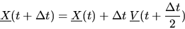
all sites  in the body. The translational motion can be integrated
by the standard leapfrog algorithm.
in the body. The translational motion can be integrated
by the standard leapfrog algorithm.
 |
(2.205) |
 |
(2.206) |
where  is the mass of the rigid unit,
  is the rigid bodies
c.o.m. velocity and
is the rigid bodies
c.o.m. velocity and  is the c.o.m. position. The cartesian
components of these quantitites are stored in the arrays: gvxx,
gvyy, and gvzz for c.o.m. velocity; and gcmx, gcmy, and gcmz for c.o.m. position.
is the c.o.m. position. The cartesian
components of these quantitites are stored in the arrays: gvxx,
gvyy, and gvzz for c.o.m. velocity; and gcmx, gcmy, and gcmz for c.o.m. position.
The torque acting upon the body in the space fixed frame is
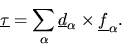 |
(2.207) |
Transformed to the local body frame (and including the centrifugal
terms) this is
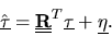 |
(2.208) |
where
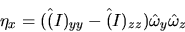 |
(2.209) |
plus cyclic permutations for  and
and  components.
The angular velocity transformed to the local body frame,
components.
The angular velocity transformed to the local body frame,
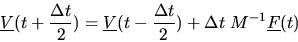
 , can then be integrated using the leapfrog algorithm and
the diagonal rotational inertia tensor.
, can then be integrated using the leapfrog algorithm and
the diagonal rotational inertia tensor.
 |
(2.210) |
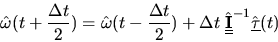
The new quaternions cannot be found so simply. DL_POLY_2 uses Fincham's
implicit quaternion algorithm (FIQA) to do this [14].
In this algorithm the new quaternions are found by solving the
implicit equation
![\begin{displaymath}
\mbox{$\underline{q}$}(t+\Delta t) = \mbox{$\underline{q}$}(...
...$}(t+\Delta t)]\hat{\mbox{$\underline{w}$}}(t+\Delta t)\right)
\end{displaymath}](img572.png) |
(2.211) |
where
![$\hat{\mbox{$\underline{w}$}} = [ 0,\hat\omega]^T$](img573.png) and
and
![$\mbox{$\underline{\underline{\bf Q}}$}[\mbox{$\underline{q}$}]$](img574.png) is
is
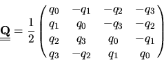 |
(2.212) |
The above equation is solved iteratively with
![\begin{displaymath}
{\mbox{$\underline{q}$}}(t+\Delta t) = {\mbox{$\underline{q}...
...}[{\mbox{$\underline{q}$}}(t)] \hat{\mbox{$\underline{w}$}}(t)
\end{displaymath}](img576.png) |
(2.213) |
as the first guess. Typically no more than 3 or 4 iterations are needed
for convergence. At each step the constraint
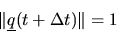 |
(2.214) |
is imposed.
The quaternions are stored in the arrays q0, q1, q2 and q3. The angular velocity (transformed to the body fixed frame) is
stored in the arrays omx, omy and omx, while the work
arrays opx, opy, opz, oqx, oqy, oqz hold values of
 and
and
 . The torques,
 are held in the work arrays tqx, tqy and tqz.
The NVE algorithm is implemented in NVEQ_1 which allows for a
system containing a mixture of rigid bodies and atomistic species,
provided the rigid bodies are not linked to other species by
constraint bonds.
Thermostats and Barostats
It is straightforward to couple the rigid body equations of motion to
a thermostat and/or barostat. The thermostat is coupled to both the
translational and rotational degrees of freedom and so both the
translational and rotational velocities are propagated in an analogous
manner to the thermostated atomic velocities. The barostat, however,
is coupled only to the translational degrees of freedom, not to the
rotational ones.DL_POLY_2 supports both Hoover type and Berendsen thermostats
and barostats for systems containing rigid bodies. The Hoover
thermostat is implemented in NVTQ/SMALL>_H1, the Hoover isotropic
barostat (plus themostat) in NPTQ/SMALL>_H1 and the anisotropic
barostat in NSTQ/SMALL>_H1. The analogous routines for the Berendsen
algorithms are NVTQ/SMALL>_B1, NPTQ/SMALL>_B1 and NSTQ/SMALL>_B1.
Next: Linked Rigid Bodies
Up: Rigid Bodies and Rotational
Previous: Description of Rigid Body
Contents
Index
W Smith
2003-05-12