Linked Rigid Bodies

The above integration algorithm can be used for rigid bodies in a system containing ``atomic'' species (whose equations of motion are integrated with the standard leapfrog algorithm). These rigid bodies may even be linked to other species (including other rigid bodies) by extensible bonds. However if a rigid body is linked to an atom or another rigid body by a bond constraint the above algorithm is not adequate. The reason is that the constraint will introduce an additional force and torque onto the body that can only be found after the integration of the unconstrained unit. DL_POLY_2 has a suite of integration algorithms to cope with this situation in which both the constraint conditions and the quaternion equations are solved similtaneously using an extension of the SHAKE algorithm called ``QSHAKE'' [15].

The QSHAKE algorithm proceeds as follows: Consider the figure in which two rigid bodies are linked by a constraint bond. We seek to choose $\mbox{$\underline{F}$}_{\rm const}$ so that at the end of the integration step the two sites in the constraint bond are a distance $r$ apart. The integration of the bodies as free units leaves the sites $r^\prime$ apart. Since the constraint force produces both a force and torque on the rigid units the correction to the constrained sites position must include both the translation and rotation of the body as a whole. The translational contribution is

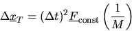$$\Delta \mbox{$\underline{x}$}_T = {(\Delta t)^2 \mbox{$\underline{F}$}_{\rm const}} \left( {1\over M} \right)$$ (2.215)

The torque induced by the constraint force is

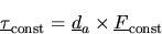$$\mbox{$\underline{\tau}$}_{\rm const} = \mbox{$\underline{d}$}_a \times \mbox{$\underline{F}$}_{\rm const}$$ (2.216)

so the correction to the angular velocity of the body is

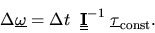$$\Delta\mbox{$\underline{\omega}$} = \Delta t \;\; \mbox{$\un... ...rline{\bf I}}$}^{-1} \; \mbox{$\underline{\tau}$}_{\rm const}.$$ (2.217)

The ``rotational'' correction to the position of the site is thus

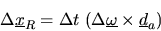$$\Delta \mbox{$\underline{x}$}_R = \Delta t\;( \Delta\mbox{$\underline{\omega}$} \times \mbox{$\underline{d}$}_a)$$ (2.218)

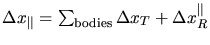
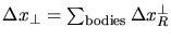
which in general will not be in the same direction as $\mbox{$\underline{F}$}_{\rm const}$ and $\Delta\mbox{$\underline{x}$}_T$. If we denote the components of $\Delta\mbox{$\underline{x}$}_R$ parallel and perpendicular to $\mbox{$\underline{F}$}_{\rm const}$ by $\Delta \mbox{$\underline{x}$}_R^\parallel$ and $\Delta \mbox{$\underline{x}$}_R^\perp$ the correction to the site position is

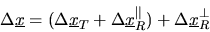$$\Delta\mbox{$\underline{x}$} = (\Delta\mbox{$\underline{x}$}... ...line{x}$}_R^\parallel) + \Delta \mbox{$\underline{x}$}_R^\perp$$ (2.219)

Clearly the presence of the constraint force and torque will mean the positions and velocities of the remaining sites in the rigid body will also have to be corrected. We proceed by seeking an approximation to $\mbox{$\underline{F}$}_{\rm const}$ then reintegrating the rigid body equations of motion with the improved total forces and torques on the body. A few iterations are normally sufficient to achieve convergence: If we assume the bond distance $r$ is large in comparison to the correction then after the correction is made the bond length is

$$r^* = \surd\left[ \left(r^\prime + \Delta x_\parallel\right)^2 + \left( \Delta x_\perp\right)^2\right]$$

$$= \surd\left[(r^{\prime})^2 + 2r^{\prime} \Delta x_{\parallel} + \Delta x_{\parallel}^2 + \Delta x_{\perp}^2 \right]$$

$$\approx \surd\left[(r^{\prime})^2 + 2r^{\prime} \Delta x_{\parallel}\right]$$ (2.220)

where $\Delta x_{\parallel} = \sum_{\rm bodies} \Delta x_T + \Delta x_R^\parallel$ and $\Delta x_{\perp} = \sum_{\rm bodies} \Delta x_R^{\perp}$. Thus a first order correction to the position of the constrained site is

$$\Delta\mbox{$\underline{x}$} = \Delta\mbox{$\underline{x}$}_T + \Delta\mbox{$\underline{x}$}_R^\parallel$$

$$= { ( \Delta t)^2 \mbox{$\underline{F}$}_{\rm const}} \left\{ { 1\o... ... \times \mbox{$\underline{d}$}_a \right]\cdot \mbox{$\underline{e}$} \ \right\}$$ (2.221)

where $\mbox{$\underline{e}$}$ is the unit vector $\mbox{$\underline{F}$}_{\rm const}/\Vert\mbox{$\underline{F}$}_{\rm const}\Vert$. The term in the $\{\ldots\}$ defines an effective mass, $\cal M$: where $1/{\cal M} = 1/ M + \left[ \left(\mbox{$\underline{\underline{\bf I}}$}^{-1}\le... ...ght)\right) \times \mbox{$\underline{d}$}_a \right]\cdot \mbox{$\underline{e}$}$.

The effective reduced mass for the two linked bodies, $a$ and $b$, is $\mu = {\cal M}_a {\cal M}_b / ({\cal M}_a + {\cal M}_b)$. As in the standard SHAKE algorithm, the reduced mass can then be used to predict the constraint force

$$F_{\rm const} = {\mu\over \Delta t^2} {{(r^2 - {r^\prime}^2)}\over 2 r^2}$$ (2.222)

Note that each prediction of the constraint force requires the rigid body equations of motion to be reintegrated accurately. If two bodies are linked by one constraint bond only two or three iterations are necessary for convergence. However convergence may be slower if an extended network of linked bodies is involved. Note also that the reduced mass needs to be re-evaluated every time-step because it depends on the relative orienation of the two bodies. Finally, we note the algorithm reduces to the standard SHAKE algorithm if the rigid bodies are replaced by point atoms. In such a case, even though $d_{a}$ is zero, care must be taken to avoid the singularity arising from $\mbox{$\underline{\underline{\bf I}}$}^{-1}$.

This ``linked rigid body'' algorithm is implemented in NVEQ_2 with the QSHAKE corrections to the forces applied in QSHAKE. Again it is straightforward to couple these systems to a Hoover type or Berendsen thermostat and/or barostat. The Hoover and Berendsen thermostated versions are found in NVTQ_H2 and NVTQ_B2 respectively. The isotropic constant pressure implementations are found in NPTQ_H2 and NPTQ_B2, while the anisotropic constant pressure routines are found in NSTQ_H2 and NSTQ_B2. An outline of the parallel version of QSHAKE is given in section 2.6.8.