Contents   Index

Integration algorithms

DL_POLY integration algorithms are based around the Verlet leapfrog scheme, which is both time reversible and simple [12]. It generates trajectories in the microcanonical (NVE) ensemble in which the total energy (kinetic plus potential energy) is conserved. If this property drifts or fluctuates excessively in the course of a simulation it indicates that the timestep is too large or the potential cutoffs too small (relative r.m.s. fluctuations in the total energy of $10^{-5}$ are typical with this algorithm).

The algorithm requires values of position $(\mbox{$\underline{r}$}$) and force ( $\mbox{$\underline{f}$}$) at time $t$ while the velocities ( $\mbox{$\underline{v}$}$) are half a timestep behind. The first step is to advance the velocities to $t+(1/2)\Delta t$ by integration of the force:

$$\mbox{$\underline{v}$}(t + {1\over 2} \Delta t) \leftarrow \... ... 2} \Delta t) + \Delta t \; {\mbox{$\underline{f}$}(t)\over m}$$ (2.173)

where $m$ is the mass of a site and $\Delta t$ is the timestep.

The positions are then advanced using the new velocities:

$$\mbox{$\underline{r}$}(t+\Delta t) \leftarrow \mbox{$\underl... ...}(t) + \Delta t \;\mbox{$\underline{v}$}(t+{1\over 2}\Delta t)$$ (2.174)

Molecular dynamics simulations normally require properties that depend on position and velocity at the same time (such as the sum of potential and kinetic energy). The velocity at time $t$ is obtained from the average of the velocities half a timestep either side of time $t$:

$$\mbox{$\underline{v}$}(t) = {1\over 2} \left[\mbox{$\underli... ...Delta t) + \mbox{$\underline{v}$}(t+{1\over 2}\Delta t)\right]$$ (2.175)

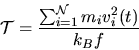
The instantaneous temperature, for example can then be obtained from the atomic velocities assuming the system has no net momentum:

$${\cal T} = {\sum_{i=1}^{\cal N} m_i v^2_i(t) \over k_B f}$$ (2.176)

where $i$ labels particles (which can be atoms or rigid molecules), ${\cal N}$ the number of particles in the system, $k_B$ Boltzmanns constant and $f$ the number of degrees of freedom in the system ($3{\cal N} - 3$ if the system is periodic and without constraints).

The routine NVE_0 implements the Verlet leapfrog algorithm and calculates the instantaneous temperature. The conserved quantity is the total energy of the system

$${\cal H}_{\rm NVE} = U + KE$$ (2.177)

where $U$ is the potential energy of the system and $KE$ the kinetic energy at time $t$.

The full selection of integrration algorithms within DL_POLY_2 is as follows:

NVE_0 		  Verlet leapfrog 

NVE_1 		  Verlet leaprog with RD-SHAKE 

NVEQ_1 		  Rigid units with FIQA and RD-SHAKE

NVEQ_2 		  Linked rigid units with QSHAKE 

NVT_B0 		  Constant T (Berendsen [16]) with Verlet leapfrog 

NVT_B1 		  Constant T (Berendsen [16]) with RD-SHAKE 

NVT_E0 		  Constant T (Evans [17]) with Verlet leapfrog 

NVT_E1 		  Constant T (Evans [17]) with RD-SHAKE 

NVT_H0 		  Constant T (Hoover [18]) with Verlet leapfrog 

NVT_H1 		  Constant T (Hoover [18]) with RD-SHAKE 

NVTQ_B1 	  Constant T (Berendsen [16]) with FIQA and RD-SHAKE 

NVTQ_B2           Constant T (Berendsen [16]) with QSHAKE 

NVTQ_H1 	  Constant T (Hoover [18]) with FIQA and RD-SHAKE 

NVTQ_H2 	  Constant T (Hoover [18]) with QSHAKE 

NPT_B0 		  Constant T,P (Berendsen [16]) with Verlet leapfrog 

NPT_B1 		  Constant T,P (Berendsen [16]) with FIQA and RD-SHAKE 

NPT_H0 		  Constant T,P+ (Hoover [18]) with Verlet leapfrog 

NPT_H1 		  Constant T,P+ (Hoover [18]) with RD-SHAKE 

NPTQ_B1 	  Constant T,P (Berendsen [16]) with FIQA and RD-SHAKE

NPTQ_B2 	  Constant T,P (Berendsen [16]) with QSHAKE 

NPTQ_H1 	  Constant T,P (Hoover [18]) with FIQA and RD-SHAKE

NPTQ_H2 	  Constant T,P (Hoover [18]) with QSHAKE 

NST_B0 		  Constant T,$\underline{\underline{\bf\sigma}}$ (Berendsen [16]) with Verlet leapfrog 

NST_B1 		  Constant T,$\underline{\underline{\bf\sigma}}$ (Berendsen [16]) with RD-SHAKE 

NST_H0 		  Constant T,$\underline{\underline{\bf\sigma}}$ (Hoover [18]) with Verlet leapfrog 

NST_H1 		  Constant T,$\underline{\underline{\bf\sigma}}$ (Hoover [18]) with RD-SHAKE 

NSTQ_B1 	  Constant T,$\underline{\underline{\bf\sigma}}$ (Berendsen [16]) with FIQA and RD-SHAKE

NSTQ_B2 	  Constant T,$\underline{\underline{\bf\sigma}}$ (Berendsen [16]) with QSHAKE 

NSTQ_H1 	  Constant T,$\underline{\underline{\bf\sigma}}$ (Hoover [18]) withFIQA and RD-SHAKE

NSTQ_H2 	  Constant T,$\underline{\underline{\bf\sigma}}$ (Hoover [18]) with QSHAKE 

In the above table the FIQA algorithm is Fincham's Implicit Quaternion Algorithm [14] and QSHAKE is the DL_POLY_2 algorithm combining rigid bonds and rigid bodies in the same molecule [15].

Subsections

• Bond Constraints
• Potential of Mean Force (PMF) Constraints and the Evaluation of Free Energy
• Thermostats
  • Nosé- Hoover Thermostat
  • Berendsen Thermostat
• Gaussian Constraints
• Barostats
  • The Hoover Barostat
  • Berendsen Barostat
• Rigid Bodies and Rotational Integration Algorithms
  • Description of Rigid Body Units
  • Integration of the Rigid Body Equations of Motion
  • Linked Rigid Bodies
• The DL_POLY_2 Multiple Timestep Algorithm
• The DL_POLY_2 RESPA Multiple Timestep Implementation

  Contents   Index